Domain-Dependent Policy Learning using Neural Networks for Classical Planning (3/4)

This third post about my undergraduate dissertation will cover my primary contributions to translate the architecture of Action Schema Networks, introduced in the previous post, for classical automated planning in the Fast-Downward framework.

The dissertation focuses on the application of ASNets in deterministic, classical planning. For this purpose, the network architecture was implemented and integrated into the Fast-Downward planning system [1] which is prominently used throughout classical planning research.

Network Definition

Prior to the integration of the network in this system, the training and evaluation, we have to define the network. As described in the previous post, the architecture of ASNets is inherently dependent on the given planning task encoded as a PDDL domain and problem specification.

PDDL in Fast-Downward

Fast-Downward itself already translates such task descriptions into planning task representations with abstracts and respective groundings. Throughout this process the tasks are also simplified and normalised removing any quantifiers, propositions which can never be fulfilled or remain constant. These steps are essential for ASNet construction as they frequently reduce the number of groundings and hence also the number of units in the proposition and action layers considerably.

Imagine a transport task with two trucks and eight locations connected in a circle, such that each location is connected to its adjacent locations. The task contains a total of eight streets, which can be driven by each truck in both directions, so it has overall $8 \cdot 2 \cdot 2 = 32$ drive actions. Naively instantiating all possible groundings would lead to $2 \cdot 8 \cdot 8 = 128$ such actions (2 trucks, 8 possible origin locations and 8 potential target locations). Similarly, the number of connected propositions, indicating whether two locations are connected, would be reduced from $8 \cdot 8 = 64$ to just 16. This has significant impact on the network size of ASNets and therefore improves their scalability.

Furthermore, these simplified task representations can be used to efficiently compute relations among grounded actions and propositions used to derive connections among ASNet layers. First, we derive the relations among the fewer abstract action schemas and predicates. For each grounding, we can then derive the respective initialisation $A$ used and apply $A$ to each respective related predicate or action schema to obtain the related groundings. This process is visualised in the table below:

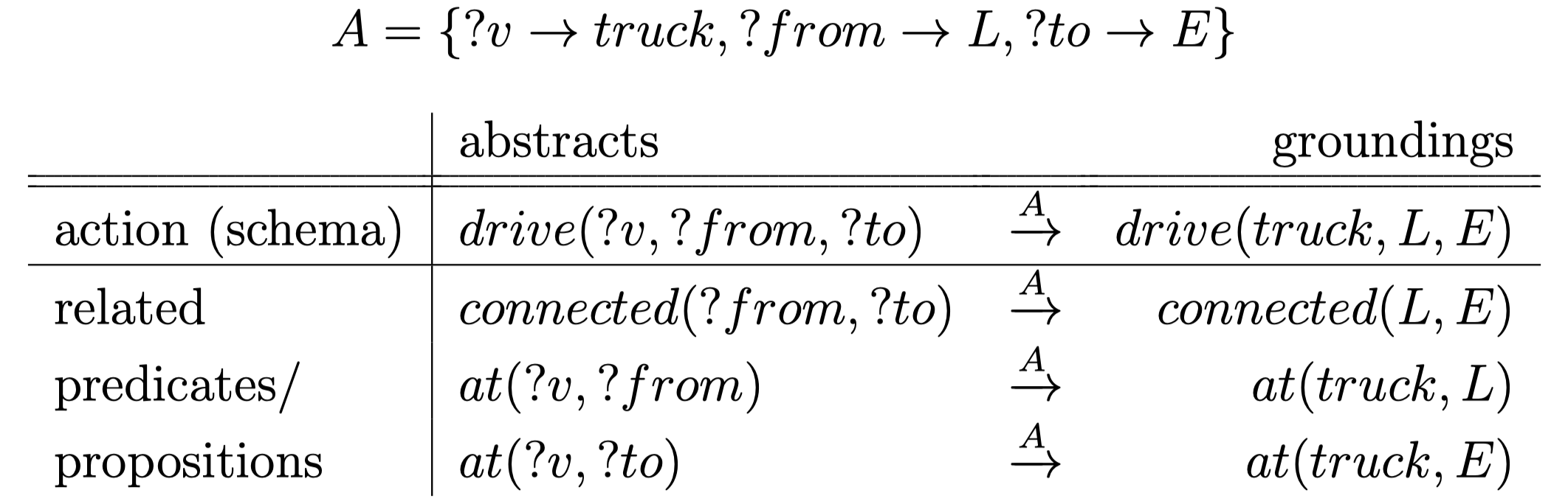
The find all propositions related to grounded action $a = drive(truck, L, E)$, we can extract the initialisation applied to obtain $a$ from the abstract action schema $drive(?v, ?from, ?to)$. This initialisation $A$ can also be applied to the related predicates of the underlying action schema to find all grounded propositions related to $a$.

Keras Network Definition

Following the creation of a planning task representation and the extraction of relations, the networks can be constructed. We defined the architecture of ASNets using Keras [2] on top of the Tensorflow [3] backend. Keras is a Python library serving as an API to multiple machine learning libraries, in our case Tensorflow, offering a modular approach with high-level abstraction. This makes Keras model definitions comparably simple to read and write as well as easily extendible. During our experiments, we used Keras version 2.1.6 with Tensorflow 1.8.0.

Generally, ASNets are structured in action and proposition layers. The respective action and proposition modules correlate to grounded actions and propositions, but their weights are shared among all modules in the layer that share the same underlying abstract action schema or predicate. Hence, we distinguished the input extraction depending on the respective grounding and the shared main module holding the weights and doing the primary computation. All such structures were implemented as custom Keras layers. Lastly, the masked softmax function to compute the output policy in the final network layer is implemented as a Keras layer to output a probability distribution over the set of actions.

Training

Training Overview

To be able to apply and exploit ASNets during planning search to solve problems of a given domain, we have to acquire knowledge and train the networks first. Such training repeatedly updates the network parameters $\theta$ including weight matrices and bias vectors with the goal of improving the network policy guidance. ASNets for a common domain can share their parameters as all problems of the same domain involve the same underlying action schemas and predicates. Therefore, it is possible to train ASNets on comparably small problem instances for a domain to obtain such parameters and exploit the obtained policy on arbitrary problem instances. This concept is essential for ASNets generalisation capability.

Sam Toyer already proposed a supervised training algorithm in his thesis [4]. However, we made minor modifications for application in deterministic, classical planning rather than probabilistic planning. Throughout training, multiple epochs are executed in which the network is trained for each given training problem in a predetermined set of training tasks $P_{train}$. For each problem, the respective network is constructed before multiple training iterations, which we refer to as problem epochs, are executed. Each such problem epoch involves the sampling of states and following update steps over the set of sampled states $\mathcal{M}$ to optimise the parameters $\theta$. Pseudocode for the entire training cycle can be seen below:

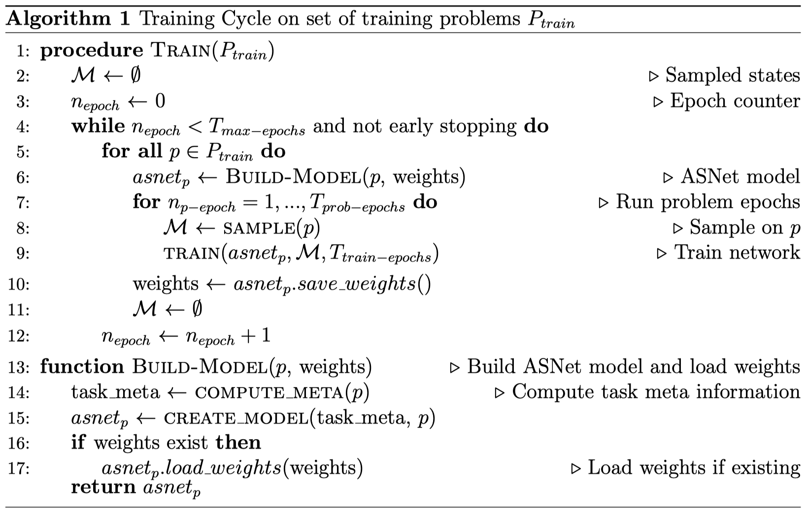
For some domains, good policies can be learned fairly easy and quickly. In these cases, it is unnecessary to execute a large number of epochs. Therefore, we potentially stop training early as proposed by Sam Toyer himself. Training is stopped early whenever a large portion of network searches during sampling successfully reached a goal and the success rate of the network search has hardly improved for multiple epochs.

Loss Function

During the training steps, the network parameters $\theta$ are updated to ensure that “good” actions are chosen in the sampled states from $\mathcal{M}$. This is achieved by optimising the parameters to minimise the following binary crossentropy loss function proposed by Sam Toyer et al. [5] $$\mathcal{L}_\theta(\mathcal{M}) = \sum_{s \in \mathcal{M}} \sum_{a \in \mathcal{A}} -(1 - y_{s,a}) \cdot log(1 - \pi^\theta(a \mid s)) - y_{s,a} \cdot log(\pi^\theta(a \mid s))$$ where $\pi^\theta(a \mid s)$ represents the probability of the network policy with parameters $\theta$ to choose action $a$ in state $s$ and $y_{s,a}$ corresponds to binary values. $y_{s,a} = 1$ if action $a$ starts an optimal plan from state $s$ onwards according to the teacher search $S^∗$. These values can be aquired during the sampling process.

Sampling

In order to enable training of the networks using the supervised algorithm described above, labelled data is needed. For ASNets in particular, such data must include state information for the network input as well as all further information required to evaluate the mentioned loss. Therefore, a sample for state $s$ can be represented by a tuple $(g, t_s, a_s, y_s)$ of four lists of binary features. The values of $g$ indicate for each fact whether it is contained in the planning task’s goal. $t_s$ shows which facts are true in $s$, $a_s$ indicates which actions are applicable in $s$ (required for the Softmax mask) and $y_s$ includes the $y_{s,a}$ values described in the loss section for each action. Note, that $g$ remains the same for all states and hence does not have to be computed for each sample. The networks will receive $g, t_s$ and $a_s$ as inputs, while the $y_{s,a}$ values are just used to compute the loss for optimisation.

Sampling Search

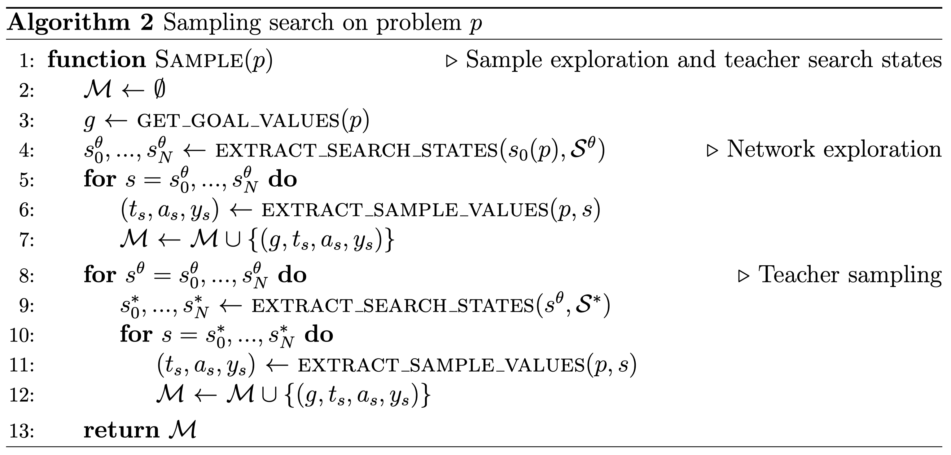
These samples are collected as part of a search applied on each planning problem in $P_{train}$. During this search we want to collect samples for states the network policy encounters to improve upon its previous performance. However, these states do not necessarily provide guidance towards the goal, especially at the beginning of training. Therefore, we also sample states along trajectories of an applied teacher search $S^*$ to ensure that the network is trained on objectively “good” states.

In the sampling search, we first explore the state space of the current problem by applying the network search $S^\theta$ which naively follows the previously constructed ASNet. Starting at the initial state $s_0$, the most probably action according to the network policy $\pi^\theta$ is followed in each state until either a dead-end, a goal or a previously encountered state is reached. The latter is required to avoid the network policy to repeatedly explore the same states as the network would apply the same actions when reaching a state for the second time. All states encountered along the explored trajectory are collected in the state memory $\mathcal{M}$.

After exploring these states based on the network policy, a predetermined teacher search $S^*$ is started from all previously collected states. Similarly to the first phase, we explore and collect states alongside the followed trajectory until a goal or dead-end is reached.

For each state $s$ collected during the sampling, the corresponding tuple $(g, t_s, a_s, y_s)$ has to be extracted. Identifying the values $g, t_s$ and $a_s$ are straight forward and only require a simple lookup of fact values in the goal set, current state and checking for applicable actions. However, obtaining the $y_{s,a}$ values is more complicated. As a reminder, these values indicate whether action $a$ starts an optimal plan from $s$ according to the teacher search $S^*$. Hence, for each sampled state we have to identify which actions start optimal plans with respect to the teacher search. First, we compute a plan from $s$ with $S^*$ and store its cost $c_s$. Then we extract the reached state $s'$ from applying $a$ in $s$ and compute the cost of the plan found for $s'$ using $S^*$. If $c_{s’} + c_a \leq c_s$ then choosing $a$ in $s$ appears to be optimal with respect to the teacher search and therefore $y_{s,a} = 1$, otherwise $y_{s,a} = 0$.

Policies in Fast-Downward

In addition to the described sampling search implemented in the Fast-Downward system [1], we also extended the system with a general framework for policies as an alternative evaluator to the usually applied heuristic functions encountered throughout automated planning.

Based on this added concept, we specifically implemented a network policy for ASNets which serves as an interface to deep learning models representing policies. This policy is based on a Fast-Downward representation of such networks responsible for extracting and feeding the required input data into the network and extracting its output. Such interaction with the networks was achieved by storing the network models as Protobuf networks.

Policy Search

Lastly, we added a new search engine based on our implementation of policies. It naively follows the most probable action for each state according to the given policy. While such a search is very simple and probably limits the achieved performance, it is solely reliant on the policy. Hence, it allows us to purely evaluate the quality of network policies. For future performance, it will certainly be of interest to apply these network policies in more sophisticated policy searches like Monte-Carlo Tree Search [6].

In the last post, I will summarise the extensive evaluation results and my concluding thoughts on this project.

References

1. Helmert, M. (2006). The Fast Downward Planning System. J. Artif. Int. Res., 26(1), 191–246. Retrieved from http://dl.acm.org/citation.cfm?id=1622559.1622565
2. Chollet, F., & others. (2015). Keras. \urlhttps://keras.io.
3. Martı́n Abadi, Ashish Agarwal, Paul Barham, Eugene Brevdo, Zhifeng Chen, Craig Citro, … Xiaoqiang Zheng. (2015). TensorFlow: Large-Scale Machine Learning on Heterogeneous Systems. Retrieved from https://www.tensorflow.org/
4. Toyer, S. (2017). Generalised Policies for Probabilistic Planning with Deep Learning (Research and Development, Honours thesis). Research School of Computer Science, Australian National University.
5. Toyer, S., Trevizan, F. W., Thiébaux, S., & Xie, L. (2017). Action Schema Networks: Generalised Policies with Deep Learning. CoRR, abs/1709.04271. Retrieved from http://arxiv.org/abs/1709.04271
6. Coulom, R. (2007). Efficient Selectivity and Backup Operators in Monte-Carlo Tree Search. In Proceedings of the 5th International Conference on Computers and Games (pp. 72–83). Turin, Italy. Retrieved from http://dl.acm.org/citation.cfm?id=1777826.1777833