Domain-Dependent Policy Learning using Neural Networks for Classical Planning (1/4)

I have finished my undergraduate Bachelor studies last summer and as a start to this blog I will outline the work I did for my dissertation titled Domain-Dependent Policy Learning using Neural Networks in Classical Planning I will split this summary over four posts which will mostly be constructed of paragraphs of my thesis, summaries of such or parts of the kolloquium presentation I held at the group seminar of the Foundations of Artificial Intelligence (FAI) group at Saarland University.

TL;DR: I transferred and applied a neural network architecture called Action Schema Networks, designed for policy learning for probabilistic planning, to deterministic, classical planning and evaluated its performance.

Introduction

Machine learning (ML) is a subfield of artificial intelligence (AI) which received tremendous media and research attention over the last years. While these terms are frequently used as if they were synonyms, such usage is misleading. ML specifically covers branches of AI involving some form of learning, mostly from large sets of data, while AI is more broad and general. It therefore aims to solve one of the main remaining challenges of computers, their limitation to obtain and rationally apply knowledge. This is arguably the main reason why humans are still superior to computers in many tasks despite their gradually increasing computational power.

The success of ML can already be seen in applications just as Alpha Go [1] and Alpha Go Zero [2], Google Deepmind’s agents, capable of beating human professionals at the Chinese board game Go. This achievement was assumed to still be decades from reality due to the game’s computational complexity constructed by its $\sim 10^{170}$ different board states [3,4]. For comparisons, it is assumed that the observable universe has about $10^{80}$ atoms. In the core of these programs were neural networks, which are often referred to under the title of deep learning, combined with algorithms from or at least related to automated planning, another field of AI with the big goal of creating an intelligent agent capable of efficiently solving (almost) arbitrary problems. While this sounds like a vision far in the future, modern planning systems are already able to solve a wide variety of tasks, e.g. complex scheduling tasks.

However, it might be surprising that planning has seen little interaction with the field of machine learning despite its rise in popularity. Only in recent past, these two fields were combined with mixed success. One of these combinational approaches was the work of Toyer et al. from the Australian National University who recently proposed a new neural network structure designed for application in probabilistic and classical automated planning, called Action Schema Networks (ASNets) [5, 6]. These are able to learn domain-specific knowledge in planning and apply it to unseen problems of the same domain. The promising structure was primarily introduced and evaluated with respect to probabilistic planning.

Therefore, the goal of my dissertation was to evaluate the possible performance of Action Schema Networks in classical planning. The main contribution of the thesis was the implementation of this novel neural network structure in the Fast-Downward planning system [7] for application in deterministic, classical planning with necessary extensions to the framework and an extensive empirical evaluation was conducted to assess ASNets on multiple tasks of varying complexity. This evaluation considered different configurations to in the end state whether Action Schema Networks are a suitable method for classical planning and if so under which conditions aiming towards the goal of learning complex relations occurring in planning tasks.

Background

Classical Automated Planning

Classical automated planning focuses on finite, deterministic, fully-observable problems solved by a single agent. The predominant formalisation for planning tasks is STRIPS [8] representing such a task as $ \Pi = (\mathcal{P}, \mathcal{A}, c, I, G) $:

• $ \mathcal{P} $ is a set of propositions (or facts)

• $ \mathcal{A} $ is a set of actions where each action $ a \in \mathcal{A} $ is a triple $ (pre_a , add_a , del_a) $ with $ pre_a, add_a , del_a \subseteq \mathcal{P} $ including a’s preconditions, add list and delete list with $ add_a \cap del_a = \emptyset $

  • preconditions are facts, which have to be true for $ a $ to be applicable

  • add list contains all propositions becoming true after applying $ a $

  • delete list contains all propositions becoming false after applying $ a $

• $ c : A \rightarrow \mathbb{R}^+_0 $ is the cost function assigning all actions to their cost

• $ I \subseteq \mathcal{P} $ is the initial state containing all propositions, which are true at the start of the task

• $ G \subseteq \mathcal{P} $ is the goal with all facts which have to become true to solve the task

Brief Example

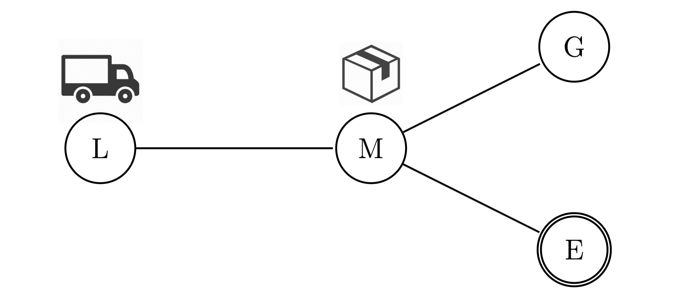
For example, one could describe a transportation task, as illustrated above, in which a truck has to deliver a package from some location to its destination by driving along streets and load or unload packages. In this concrete example, the truck has to drive from London (L) to Manchester (M), pick up the package, drive to Edinburgh (E) and unload the package there. The task would include the propositions $\mathcal{P} = \{at(o, x) \mid o \in \{t, p\}, x \in \{L, M, G, E\}\}$ and actions $\mathcal{A} = \{drive(x, y, z) \mid x \in \{truck\}; y, z \in \{L, M, G, E\}; y \text{ and } z \text{ are connected}\} \cup \{load(x, y, z), unload(x, y, z) \mid x \in \{truck\}, y \in \{package\}, z \in \{L, M, G, E\}\}$. The goal could be formalised as $ \{at(package, E)\} $ and the initial state describes the starting position of the truck and package as $\{at(truck, L), at(package, M)\}$.

To solve any task $\Pi$ in automated planning, the planner has to observe the current state and choose actions, one at a time, in order to reach a goal state $s^*$ with $G \subseteq s^∗$. The sequence of actions, applied to get to such a state, is called plan for $\Pi$. A plan is considered optimal if it has the least cost out of all plans reaching a goal. E.g., the optimal plan for our transport task would be $ \langle drive(truck, L, M), load(truck, package, M), drive(truck, M, E), unload(truck, package, E) \rangle $.

Modelling - PDDL

One essential component of planning is to model the task at hand. This process is usually split into two components: the domain and problem. This separation has its origin in the main modelling language for planning PDDL (Planning Domain Definition Language) introduced by McDermott et al. [9]. A domain describes a whole family of various problems sharing the core idea. It contains predicates defined on abstract objects as well as action schemas. Problem instances are always assigned a domain which predefines mentioned elements. In the problem file concrete objects are defined instantiating the predicates and action schemas of the domain to propositions and actions respectively. Furthermore the initial and goal states are specified.

Most of these planning problems seem conceptually easy for rational-thinking humans, but this impression can be misleading. In fact, planning is computationally extremely difficult. Merely deciding whether a task is solvable is already PSPACE-complete [10].

Deep Learning

Foundation

The idea of neural networks (NNs) has a long history reaching back to the 1940s [11] inspired by the human brain whose immensely impressive capabilities are partly due to the dense connectivity of neurons. With the introduction of the perceptron, which was capable of learning, by F. Rosenblatt in 1958 [12] and backpropagation by Rumelhart et al. in 1986 [13] the foundation for modern NNs was built.

The simplest, modern NN architecture is the fully-connected feedforward network or multi-layer perceptron (MLP) as illustrated below. As (almost) all neural network architectures, it consists of various layers containing nodes or units which are successively connected with each other. One usually speaks of input layer (yellow), hidden layers (blue) and an output layer (green). Each connection of two nodes is weighted with a parameter.

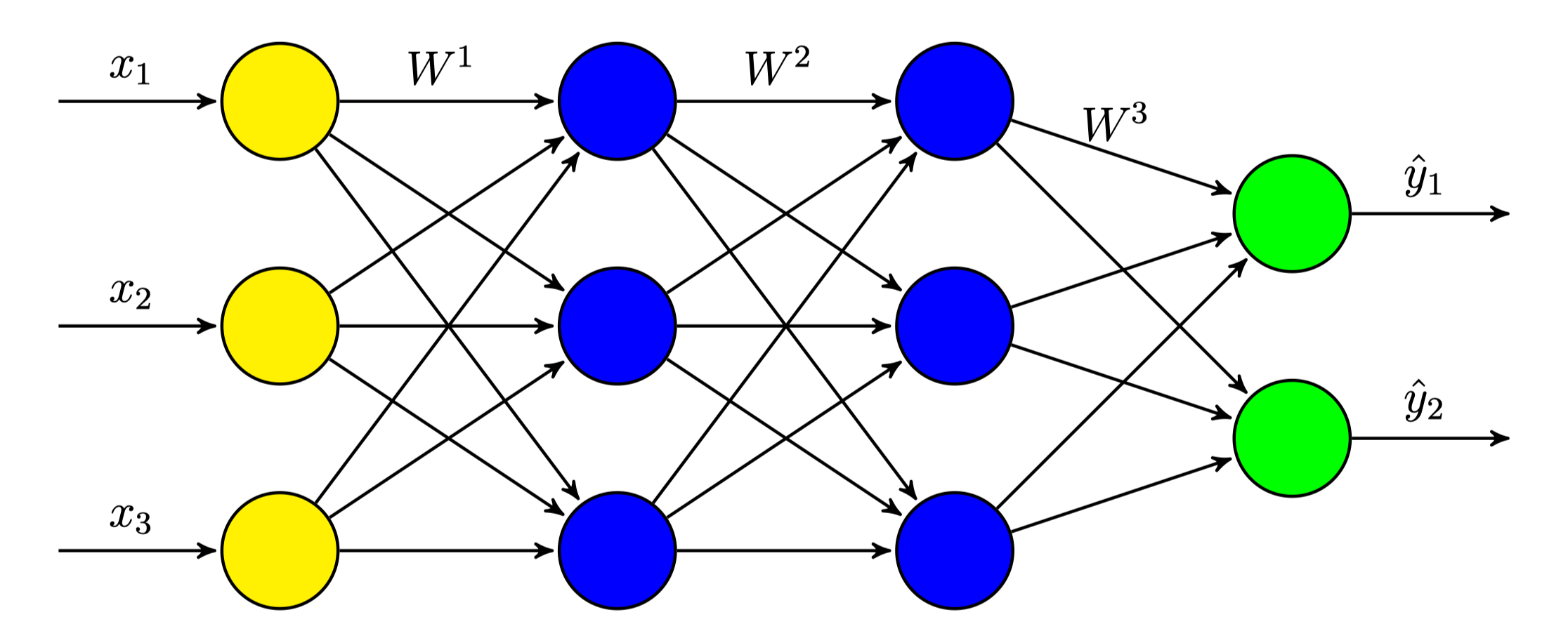
A node is usually computing a fairly simple mathematical operation in which it applies the weights to each input of the previous layer, adds a bias vector and finally applies a nonlinear function $ f $, often called activation function. The output of the $ l $-th layer $ h^l $ can therefore be computed as follows:

$$ h^l = f(W^l \cdot h^{l-1} + b^l) $$

The weights and bias vectors are collectively stored and form the “learned intelligence” of these networks gradually optimised with respect to some goal. The objective is usually represented by a loss function $ L(\hat{y}, y) $ depending on the true output $ y $ and the prediction $ \hat{y} $ computed by the network for a given input $ x $. This form of training is called supervised learning and depends on labelled training data including inputs as well as their expected output. The optimisation is usually achieved by gradient-descent in which all parameters, annotated as $ \theta $, are updated in the direction of the steepest descent of the loss function $ L $ for some step-size $ \alpha $, called learning rate:

$$ \theta = \theta - \alpha \nabla_\theta L(\hat{y}, y) $$

Convolutional Neural Networks

Over the last few years, many different architectures of such networks evolved with specific applications. Recurrent neural networks (RNNs) are capable of considering past knowledge and decisions and therefore incorporate something similar to a memory. This property turned out especially valuable whenever processing language reaching state-of-the-art in tasks as machine translation [14, 15] and speech recognition [16].

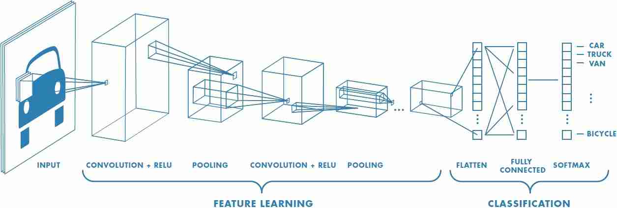
Similarly, convolutional neural networks (CNNs) became the standard for many multi-dimensional, mostly visual, input tasks reaching unseen accuracy in e.g. image classification [17]. The main characteristic of CNNs is the application of the mathematical convolution operation. This linear operation replaces the typical matrix multiplication known from MLPs where every unit in each layer has a weighted connection to every node in the successive layer. In convolution, smaller weight matrices, called filters or kernels, are applied by “sliding” the filters over the units in one layer with each applying its operation to a set of neighboured inputs. This form of processing brings multiple advantages.

Due to the usually smaller size of filters, CNNs have sparse connectivity, only combining neighboured units in one operation. This makes use of local properties to extract input features like edges in visual domains, which is especially meaningful in deep CNNs. While shallow layers detect e.g. edges or shapes of an input image, filters in deeper layers could work upon these features and detect increasingly abstract objects like cars and humans.

Additionally, filters are reused repeatedly during the “sliding”, applying their operation to (partially) different input units. This form of weight sharing allows to significantly reduce the amount of parameters needed. Hence, the memory requirements of the networks are lowered, making them more efficient than fully-connected NNs because less parameters have to be learned, so needed training time and data can be reduced by the approach.

In the next post, I will outline ASNets as a network structure before explaining my adjustments for application in classical planning as well as the results of the evaluation in the third and forth part.

References

1. Silver, D., Hubert, T., Schrittwieser, J., Antonoglou, I., Lai, M., Guez, A., … Hassabis, D. (2017). Mastering Chess and Shogi by Self-Play with a General Reinforcement Learning Algorithm. ArXiv e-Prints.
2. Müller, M. (2002). Computer go. Artificial Intelligence, 134(1-2), 145–179.
3. Tromp, J., & Farnebäck, G. (2006). Combinatorics of go. In International Conference on Computers and Games (pp. 84–99). Springer.
4. Toyer, S. (2017). Generalised Policies for Probabilistic Planning with Deep Learning (Research and Development, Honours thesis). Research School of Computer Science, Australian National University.
5. Toyer, S., Trevizan, F. W., Thiébaux, S., & Xie, L. (2017). Action Schema Networks: Generalised Policies with Deep Learning. CoRR, abs/1709.04271. Retrieved from http://arxiv.org/abs/1709.04271
6. Helmert, M. (2006). The Fast Downward Planning System. J. Artif. Int. Res., 26(1), 191–246. Retrieved from http://dl.acm.org/citation.cfm?id=1622559.1622565
7. Fikes, R. E., & Nilsson, N. (1971). STRIPS: A New Approach to the Application of Theorem Proving to Problem Solving. Ai, 2, 189–208.
8. McDermott, D., & others. (1998). The PDDL Planning Domain Definition Language. The AIPS-98 Planning Competition Comitee.
9. Bylander, T. (1994). The Computational Complexity of Propositional STRIPS Planning. Ai, 69(1–2), 165–204.
10. McCulloch, W., & Pitts, W. (1986). A Logical Calculus of the Ideas Immanent in Nervous Activity. Brain Theory, 229–230.
11. Rosenblatt, F. (1958). The perceptron: A probabilistic model for information storage and organization in the brain. Psychological Review, 64(6), 386–408.
12. Rumelhart, D. E., Hinton, G. E., & Williams, R. J. (1988). Neurocomputing: Foundations of Research. In J. A. Anderson & E. Rosenfeld (Eds.) (pp. 696–699). Cambridge, MA, USA: MIT Press. Retrieved from http://dl.acm.org/citation.cfm?id=65669.104451
13. Bahdanau, D., Cho, K., & Bengio, Y. (2014). Neural machine translation by jointly learning to align and translate. ArXiv Preprint ArXiv:1409.0473.
14. Cho, K., Van Merriënboer, B., Gulcehre, C., Bahdanau, D., Bougares, F., Schwenk, H., & Bengio, Y. (2014). Learning phrase representations using RNN encoder-decoder for statistical machine translation. ArXiv Preprint ArXiv:1406.1078.
15. Graves, A., Mohamed, A.-rahman, & Hinton, G. (2013). Speech recognition with deep recurrent neural networks. In Acoustics, speech and signal processing (icassp), 2013 ieee international conference on (pp. 6645–6649). IEEE.
16. Krizhevsky, A., Sutskever, I., & Hinton, G. E. (2012). ImageNet Classification with Deep Convolutional Neural Networks. In F. Pereira, C. J. C. Burges, L. Bottou, & K. Q. Weinberger (Eds.), Advances in Neural Information Processing Systems 25 (pp. 1097–1105). Curran Associates, Inc. Retrieved from http://papers.nips.cc/paper/4824-imagenet-classification-with-deep-convolutional-neural-networks.pdf